Expected number of faces in Gaussian polytopes

Last week I was reading Active Learning via Perfect Selective Classification by El-Yaniv and Wiener, and came across a neat result due to Hug and Reitzner that they use in some of their bounds for active learning on Gaussian distributions.

The setup is the following : let X_1, X_2, \ldots, X_n be n jointly Gaussian vectors with distribution \mathcal{N}(0,I_d) in \mathbb{R}^d. The convex hull P_n of these points is called a Gaussian polytope. This is a random polytope of course, and we can ask various things about their shape : what is the distribution of the number of vertices, or the number of k-faces? Let f_k(P_n) be the number of k-faces Distributions are hard, but for general k the expected number of faces (as n \to infty) is given by

\mathbb{E}[ f_k(P_n)] = \frac{2^d}{\sqrt{d}} \binom{d}{k+1} \beta_{k,d-1}(\pi \ln n)^{(d-1)/2} (1 + o(1)),

where \beta_{k,d-1} is the internal angle of a regular (d-1)-simplex at one of its k-dimensional faces. What Hug and Reitzner show is a bound on the variance (which then El-Yaniv and Plan use in a Chebyshev bound) : there exists a constant c_d such that

\mathrm{Var}( F_k(P_n) ) \le c_d (\ln n)^{(d-1)/2}

So the variance of the number of k-faces can be upper bounded by something that does not depend at all on the actual value of k. In fact, they show that

f_k(P_n) (\ln n)^{-(d-1)/2} \to \frac{2^d}{\sqrt{d}} \binom{d}{k+1} \beta_{k,d-1} \pi^{(d-1)/2}

in probability as n \to \infty. That is, appropriately normalized, the number of faces converges to a constant.

To me this result was initially surprising, but after some more thought it makes a bit more sense. If you give me a cloud of Gaussian points, then I need k+1 points to define a k-face. The formula for the mean says that if I chose a random set of k+1 points, then approximately \frac{2^d}{\sqrt{d}} \beta_{k,d-1}(\pi \ln n)^{(d-1)/2} fraction of them will form a real k-face of the polytope. This also explains why the simplex-related quantity appears — points that are on “opposite sides” of the sphere (the level sets of the density) are not going to form a face together. As n \to \infty this fraction will change, but effectively the rate of growth in the number of faces with n is (\ln n)^{(d-1)/2}, regardless of k.

I’m not sure where this result will be useful for me (yet!) but it seemed like something that the technically-minded readers of the blog would find interesting as well.

C.R. Rao and information geometry

On Lalitha’s recommendation I read Frank Nielsen’s paper “Cramer-Rao Lower Bound and Information Geometry,” which is a survey how C.R. Rao’s work has impacted information geometry. I remember spending some time in grad school trying to learn information geometry (mostly for fun), but since it ended up not being particularly useful in my research, I’m afraid a lot of it has leaked out of my ears. This paper has a short introduction to the Cramer-Rao lower bound and an introduction to information geometry which might be a nice read for some of the readers of this blog. It’s certainly faster than trying to read Amari’s monograph! In particular, it goes over the “highlights” of geodesics and other geometric features on the manifold of probability distributions.

The paper mentions the sub-family of f-divergences known as \alpha-divergences, which are given by

D_{\alpha}(p \| q) = \frac{4}{1 - \alpha^2} \left( 1 - \int p(x)^{(1 - \alpha)/2)} q(x)^{(1 + \alpha)/2} dx \right)

The KL divergence is D_{-1}(p \| q) — you have to take the limit as \alpha \to -1. Within this family of divergences we have the relation D_{\alpha}(p \| q) = D_{-\alpha}(q \| p). Consider a pair of random variables (X,Y) with joint distribution P_{XY} and marginal distributions P_X and P_Y. If we take q = P_X P_Y and p = P_{XY} then the mutual information is D_{-1}( p \| q ). But we can also take

D_{-1}( P_{X} P_{Y} \| P_{XY}) = D_1( P_{XY} \| P_{X} P_{Y} )

Thus it turns out that the “lautum information” defined by Palomar and Verdú is a special case of this: it’s the 1-divergence between the the joint distribution and the product of the marginals. While their paper mentions the lautum information is an f-divergence, it doesn’t discuss this connection to this family of divergences. Nielsen’s paper calls this the “reverse Kullback-Leibler divergence,” but some googling doesn’t seem to indicate that this is a common term, or indeed if it has some use in information geometry. Palomar and Verdú give several operational interpretations of the lautum information.

Linkage

Quicksort as a dance. Via James Fallows.

I have a subscription to Harper’s and try to solve the cryptic crossword each month in the vain hope that I will win a free year’s subscription. The puzzles back to 1976 have been posted online.

Tesla and the lone inventor myth.

My friend (and ex-fellow actor) Stephen Larson‘s project OpenWorm was written up in Wired UK.

Max has an important reminder about stochastic kernels and conditional probabilities.

Generating vector-valued noise for differential privacy

A distribution that appears frequently in differential privacy is the Laplace distribution. While in the scalar case we have seen that Laplace noise may not be the best, it’s still the easiest example to start with. Suppose we have n scalars x_i \in [0,1] and we want to compute the average \frac{1}{n} \sum_{i} x_i in a differentially private way. One way to do this is to release
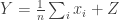
 Y = \frac{1}{n} \sum_{i} x_i + Z, where Z has a Laplace distribution:

p(z) = \frac{\lambda}{2} \exp( - \lambda |z| ).

To see that this is differentially private, note that by changing one value of x_i the average can change by at most \pm \frac{1}{n}. Let \bar{x} and \bar{x}' be the average of the original data and the data with one element changed. The output density in these two cases has distribution p( y - \bar{x}) and p(y - \bar{x}'), so for a

\frac{ p(y - \bar{x}) }{ p(y - \bar{x}') } \le \exp( \lambda ( |y - \bar{x}'| - |y - \bar{x}| ) ) \le \exp( \lambda |\bar{x} - \bar{x}|' ) \le \exp( \lambda/n )

So we can see by choosing \lambda = n \epsilon we get an \epsilon-differentially private approximation to the average.

What if we now have n vectors \mathbf{x}_i \in [0,1]^d? Well, one candidate is release a differentially private version of the mean by computing \mathbf{Y} = \frac{1}{n} \sum_{i} \mathbf{X}_i + \mathbf{Z}, where \mathbf{Z} has a distribution that looks Laplace-like but in higher dimensions:

p(\mathbf{z}) \propto \exp( - \lambda \| \mathbf{z} \| )

Now we can do the same calculation with means \bar{\mathbf{x}} and \bar{\mathbf{x}}'

\frac{ p(\mathbf{y} - \bar{\mathbf{x}}) }{ p(\mathbf{y} - \bar{\mathbf{x}}') } \le \exp( \lambda ( \|\mathbf{y} - \bar{\mathbf{x}}'\| - \|\mathbf{y} - \bar{\mathbf{x}}\| ) ) \le \exp( \lambda \|\bar{\mathbf{x}} - \bar{\mathbf{x}}'\| )

Now the Euclidean norm of the average vector can change by a most \sqrt{d}/n (by replacing x_i = \mathbf{0} with x_i' = \mathbf{1}, for example), so the overall bound is \exp(\lambda \sqrt{d}/n), which means choosing \lambda = n \epsilon / \sqrt{d} we get \epsilon-differential privacy.

Sampling from exponentials is easy, but what about sampling from this distribution? Here’s where people can fall into a trap because they are not careful about transformations of random variables. It’s tempting (if you are rusty on your probability) to say that

p(\mathbf{z}) = C(\lambda) \exp( - \lambda \| \mathbf{z} \| )

and then say “well, the norm looks exponentially distributed and the direction is isotropic so we can just sample the norm with an exponential distribution and the uniform direction by taking i.i.d. Gaussians and normalizing them.” But that’s totally wrong because that is implicitly doing a change of variables without properly adjusting the density function. The correct thing to do is to change from Euclidean coordinates to spherical coordinates. We have a map T : (z_1, z_2, \ldots, z_d) \to (r, \phi_1, \phi_2, \ldots, \phi_{d-1}) whose Jacobian is

J(r, \phi_1, \phi_2, \ldots, \phi_{d-1}) = r^{d-1} \sin^{d-2}(\phi_1) \ldots, \sin(\phi_{d-2}).

Plugging this in and noting that r = \|\mathbf{z}\| we get

p(r, \phi_1, \phi_2, \ldots, \phi_{d-1}) = C'(\lambda,\phi_1,\ldots, \phi_{d-1}) \exp( - \lambda r ).

So now we can see that the distribution factorizes and indeed the radius and direction are independent. The radius is not exponentially distributed, it’s Erlang with parameters (d,\lambda). We can generate this by taking the sum of d exponential variables with parameter \lambda. The direction we can pick uniformly by sampling d i.i.d. Gaussians and normalizing them.

In general sampling distributions for differentially private mechanisms can be complicated — for example in our work on PCA we had to use an MCMC procedure in our experiments to sample from the distribution in our algorithm. This means we could really only approximate our algorithm in the experiments, of course. There are also places to slip up in sampling from simple-looking distributions, and I’d be willing to bet that in some implementations out there people are not sampling from the correct distribution.

(Thanks to Kamalika Chaudhuri for inspiring this post.)

Some not-so-recent ArXiV skims

I tend to flag papers on ArXiV that I want to take a look at in (soon to be defunct, *sniff*) Google Reader. Here are some papers from the last month that I found interesting. I’ll post a few more of these as I work through my backlog…

Local Privacy and Statistical Minimax Rates (John C. Duchi, Michael I. Jordan, Martin J. Wainwright) — this is a paper proving minimax lower bounds for differential privacy. The approach is based on the Fano/Le Cam style of getting minimax bounds by constructing a packing of instances of the problem.

Bernstein – von Mises Theorem for growing parameter dimension (Vladimir Spokoiny) — I’m generally interested in the consistency properties of Bayesian procedures, and this looks at the effect of asymptotically growing the problem size to see how fast the problem can grow while still getting the same consistency from the BvM theorem.

On the problem of reversibility of the entropy power inequality (Sergey G. Bobkov, Mokshay M. Madiman) — More results on the EPI. Reversing it is the same as reversing the Brunn-Minkowski inequality (consider uniform distributions), but there is an interesting impossibility result here (Theorem 1.3): “For any constant C, there is a convex probability distribution \mu on the real line with a finite entropy, such that \min \{ H(X+Y), H(X-Y) \} \ge C H(X), where X and Y are independent random variables, distributed according to \mu.” The distribution they use is a truncated Pareto distribution but the calculations seem hairy.

A universal, operational theory of unicast multi-user communication with fidelity criteria (Mukul Agarwal, Sanjoy Mitter, Anant Sahai) — This is the culmination of Mukul’s work starting from a very nice paper I cite all the time from Allerton. There are several results and commentary in here — there’s a fair bit of philosophy, so it’s worth a more patient read than I could give it so far (only so many hours in the day, after all!)

The Convergence Rate of Majority Vote under Exchangeability (Miles E. Lopes) — The title says it all, really. The bounds are actually in terms of the mixture distribution of the exchangeable sequence of Bernoulli votes.

Paper a day(?) : optimal mechanisms for differential privacy

Maybe more like “paper whenever I feel like it.” This is a post on a now not-so-recent ArXiV preprint by Quan Geng and Pramod Viswanath on constructing the best mechanism (output distribution) for guaranteeing differential privacy under a utility constraint.

Continue reading

Linkage (technical)

Having seen a talk recently by John Ioannidis on how medical research is (often) bunk, this finer corrective by Larry Wasserman was nice to read.

Computer science conferences are often not organized by the ACM, but instead there are different foundations for machine learning and vision and so on that basically exist to organize the annual conference(s). At least, that is what I understand. There are a few which are run by the ACM, and there’s often debate about whether or not the ACM affiliation is worth it, given the overheads and so on. Boaz Barak had a post a little over a week ago making the case for sticking with the ACM. Given the hegemonic control of the IEEE on all things EE (more or less), this debate is new to me. As far as I can tell, ISIT exists to cover some of the cost of publishing the IT Transactions, and so it sort of has to be run by IEEE.

As mentioned before, Tara Javidi has a nice post up on what it means for one random variable to be stochastically less variable than another.

Paul Miniero has a bigger picture view of NIPS — I saw there were lots of papers on “deep learning” but it’s not really my area so I missed many of those posters.

David Eppstein’s top 10 cs.DS papers from 2012.

Linkage (technical)

Here’s a roundup of some interesting posts/pages on technical things.

Over at Larry Wasserman’s blog, Rob Tibshirani suggests 9 Great Statistics papers published after 1970. You know, in case you were looking for some light reading over winter break.

Videos from the DIMACS Differential Privacy Workshop are up.

All of these ads for jobs this year want someone who works on Big Data. But… do you really have big data? Or, as I like to ask, “how big is big, anyway?”

Speaking of big data, this talk by Peter Bartlett looks cool. (h/t Andrew Gelman)

Max Raginsky and Igal Sason have a tutorial on measure concentration. Log Sobolev inequalities are a dish best served cold.

I’ll probably do an ArXiV roundup sometime soon — trying to catch up on a backlog of reading and thinking lately.

Collisions from entropy bounded random variables

I realized the other day that for two completely unrelated papers I’ve had to prove statements about how many unique elements appear in a sample from distribution P on a discrete set. The thing is we only have a handle on the entropy H(P) but not on the distribution itself.

Let P have entropy H(P) and consider a sample of size m drawn i.i.d. from P. Let M be the number of distinct symbols in the sample. Then
\mathbb{E}[M] \le \frac{m H(P)}{\log m} + 1

Let \{p_i\} be the probabilities of the different elements. There could be countably many, but we can write the expectation of the number of unique elements as
\mathbb{E}[M] = \sum_{i=1}^{\infty} (1 - (1 - p_i)^m)
By doing a bit of series manipulation you can get the bound above. This came up (perhaps unsurprisingly) in some work on large-alphabet probability estimation.

Let P have entropy H(P) and support size K and consider a sample of size n drawn i.i.d. from P. Let M be the number of distinct symbols in the sample. Then
\mathbb{P}(M = n) \ge \left( \frac{H(P) -  1 - \log n}{\log K} \right)^{n-1}

For this result we need a bound on the support of P as well, which makes things a little easier. This result came up when we were proving bound on adversarial strategies when eavesdropping. We needed to show that if P represents some sort of list-decoding based on what the adversary has seen over the channel so far, then the list has some structure/distance properties. This lemma came in handy.

I’m sure there’s a better way to clean up these kinds of results to get something more “off the shelf” for general distributions. In both cases we didn’t find these result easily somewhere else so we ended up proving them as one-off lemmas.

Juggling, (a)synchrony, and queues

Research often takes twisty little paths, and as the result of a recent attempt to gain understanding about a problem I was trying to understand the difference between the following two systems with k balls and n (ordered) bins:

  1. Synchronous: take all of the top balls in each bin and reassign them randomly and uniformly to the bottoms of the bins.
  2. Asynchronous: pick a random bin, take the top ball in that bin, and reassign it randomly and uniformly to the bottom of a bin.

These processes sound a bit similar, right? The first one is a batch version of the second one. Sort of. We can think of this as modeling customers (balls) in queues (bins) or balls being juggled by n hands (bins).

Each of these processes can be modeled as a Markov chain on the vector of bin occupation numbers. For example, for 3 balls and 3 bins we have configurations that look like (3,0,0) and its permutations, (2,1,0) and its permutations, and (1,1,1) for a total of 10 states. If you look at the two Markov chains, they are different, and it turns out they have different stationary distributions, even. Why is that? The asynchronous chain is reversible and all transitions are symmetric. The synchronous one is not reversible.

One question is if there is a limiting sense in which these are similar — can the synchronous batch-recirculating scheme be approximated by the asynchronous version if we let n or k get very large?