Paper a day(?) : optimal mechanisms for differential privacy

Posted on March 5, 2013 by Anand Sarwate

Maybe more like “paper whenever I feel like it.” This is a post on a now not-so-recent ArXiV preprint by Quan Geng and Pramod Viswanath on constructing the best mechanism (output distribution) for guaranteeing differential privacy under a utility constraint.

Continue reading →

Mean absolute deviations for binomial random variables

Posted on October 18, 2010 by Anand Sarwate

Update: thanks to Yihong Wu for pointing out a typo in the statement of the result, which then took me months to get around to fixing.

I came across this paper in the Annals of Probability:

Mean absolute deviations of sample means and minimally concentrated binomials
Lutz Mattner

It contains the following cute lemma, which I didn’t know about before. Let $S_n$ have binomial distribution with parameters $(n,p)$ . Let $b(n,k,p) = \mathbb{P}(S_n = k)$ . The first two parts of the lemma are given below.

Lemma. We have the following:

$k_0 \in \arg\max_{k \in \{0,\ldots, n\}} b(n,k,p)$ if and only if $k_0 \in \{0,\ldots, n\}$ and $(n+1)p - 1 \le k_0 \le (n+1) p$ .
(De Moivre’s mean absolute deviation equality) $\sum_{k=0}^{n} |k - np| b(n,k,p) = 2 v (1-p) \max_{k \in \{0,\ldots, n-1\}} b(n-1,k,p)$ , where $v$ is the unique integer between $np < v \le np + 1$ .

The second part, which was new to me (perhaps I’ve been too sheltered), is also in a lovely paper from 1991 by Persi Diaconis and Sandy Zabell : “Closed Form Summation for Classical Distributions: Variations on a Theme of De Moivre,” in Statistical Science. Note that the sum in the second part is nothing more than $\mathbb{E}|S_n - np|$ . Using this result, De Moivre proved that $\lim_{n \to \infty} \mathbb{E}|S_n/n - p| \to 0$ , which implied (to him) that

if after taking a great number of experiments, it should be perceived that the happenings and failings have been nearly in a certain proportion, such as of 2 to 1, it may safely be concluded that the probabilities of happening or failing at any one time assigned will be very near in that proportion, and that the greater the number of experiments has been, so much nearer the truth will the conjectures be that are derived from them.

Diaconis and Zabell show the origins of this lemma, which leads to De Moivre’s result on the normal approximation to the binomial distribution. As for the proof of the $L_1$ convergence, they call the proof in the $p = 1/2$ case “simple but clever, impressive if only because of the notational infirmities of the day.” De Moivre’s proof was in Latin, but you can read a translation in their paper. A simple proof for rational $p$ was given by Todhunter in 1865.

For those with an interest in probability with a dash of history to go along, the paper is a fun read.

paper a (long time period) : Assouad, Fano, and Le Cam

Posted on November 6, 2009 by Anand Sarwate

Kamalika pointed me to this paper by Bin Yu in a Festschrift for Lucien Le Cam. People who read this blog who took information theory are undoubtedly familiar with Fano’s inequality, and those who are more on the CS theory side may have heard of Assouad (but not for this lemma). This paper describes the relationship between several lower bounds on hypothesis testing and parameter estimation.

Suppose we have a parametric family of distributions $\mathcal{P} = \{P_{\theta} : \theta \in \mathcal{D}\}$ , where $\mathcal{D}$ is a metric space with metric $d(\cdot,\cdot)$ . For two distributions $P_1$ and $P_2$ define the affinity $\|P_1 \wedge P_2 \|$ by:

$\|P_1 \wedge P_2 \| = 1 - \frac{1}{2} \| P_1 - P_2 \|_1$

Let $\mathop{\rm co}(\cdot)$ denote the convex hull. Then Le Cam’s lemmas is the following.

Le Cam’s Lemma. Let $\hat{\theta}$ be an estimator of $\theta(P)$ on $\mathcal{P}$ . Suppose $D_1$ and $D_2$ be two sets such that $d(s_1,s_2) \ge 2 \delta$ for all $(s_1,s_2) \in D_1 \times D_2$ , and $\mathcal{P}_1$ and $\mathcal{P}_2$ be two subsets of $\mathcal{P}$ such that $\theta(P) \in D_i$ when $P \in \mathcal{P}_i$ . Then

$\sup_{P \in \mathcal{P}} \mathbb{E}_P[ d(\hat{\theta}, \theta(P)) ] \ge \delta \cdot \sup_{P_i \in \mathop{\rm co}(\mathcal{P}_i)} \| P_1 \wedge P_2 \|$

This lemma gives a lower bound on the error of parameter estimates in terms of the total variational distance between the distributions associated to different parameter sets. It’s a bit different than the bounds we usually think of like Stein’s Lemma, and also a bit different than bounds like the Cramer-Rao bound.

Le Cam’s lemma can be used to prove Assouad’s lemma, which is a statement about a more structured set of distributions indexed by the $H = \{-1, 1\}^m$ , the vertices of the hypercube. We’ll write $t \sim_j t'$ for $t,t' \in H$ if they differ in the j-th coordinate.

Assouad’s Lemma. Let $\mathcal{F}_m = \{P_{t} : t \in H\}$ be a set of $2^m$ probability measures indexed by $H$ , and suppose there are $m$ pseudo-distances $d_m$ on $\mathcal{D}$ such that for any pair $(x,y)$

$d(x,y) = \sum_{j}^m d_j(x,y)$

and that if $t \sim_j t'$

$d_j( \theta(P_t), \theta(P_{t'}) ) \ge \alpha_m$

Then

$\max_{P_t \in \mathcal{F}_m} \mathbb{E}_{t}[ d(\hat{\theta},\theta(P_t))] \ge m \cdot \frac{\alpha_m}{2} \min\{ \|P_t \wedge P_{t'} \| : t \sim_j t', j \le m\}$

The min comes about because it is the weakest over all neighbors (that is, over all j) of $P_t$ in the hypercube. Assouad’s Lemma has been used in various different places, from covariance estimation, learning, and other minimax problems.

Yu then shows how to prove Fano’s inequality from Assouad’s inequality. In information theory we see Fano’s Lemma as a statement about random variables and then it gets used in converse arguments for coding theorems to bound the entropy of the message set. Note that a decoder is really trying to do a multi-way hypothesis test, so we can think about the result in terms of hypothesis testing instead. This version can also be found in the Wikipedia article on Fano’s inequality.

Fano’s Lemma. Let $\mathcal{M}_r \subset \mathcal{P}$ contain $r$ probability measures such that for all $j \ne j'$ with $j,j' \le r$

$d(\theta(P_j), \theta(P_{j'})) \ge \alpha_r$

and

$D(P_j~\|~P_{j'}) \le \beta_r$

Then

$\max_j \mathbb{E}_j[ d(\hat{\theta},\theta(P_j)) ] \ge \frac{\alpha_r}{2}\left( 1 - \frac{\beta_r + \log 2}{\log r} \right)$

Here $D(\cdot\|\cdot)$ is the KL-divergence. The proof follows from the regular Fano’s inequality by choosing a message $W$ uniformly in $\{1, 2, \ldots, r\}$ and then setting the output $Y$ to have the distribution $P_j$ conditioned on $W = j$ .

The rest of the paper is definitely worth reading, but to me it was nice to see that Fano’s inequality is interesting beyond coding theory, and is in fact just one of several kinds of lower bound for estimation error.

paper a day : Recovery of Time Encoded Bandlimited Signals

Posted on January 14, 2008 by Anand Sarwate

Perfect Recovery and Sensitivity Analysis of Time Encoded Bandlimited Signals
Aurel A. Lazar and László T. Tóth
IEEE Transactions on Circuits and Systems – I: Regular Papers, vol. 51, no. 10, October 2004

I heard about this paper from Prakash Narayan, who came to give a seminar at last semester, and I thought it was pretty interesting. In an undergrad signals and systems class we usually spend most of our time talking about converting an analog signal x(t) into a discrete-time signal x[n] by sampling x(t) regularly in time. That is, we set x[n] = x(nT) for some sampling interval T. There are at least two reasons for doing things this way: it’s simple to explain and the math is beautiful. If x(t) is a bandlimited signal, it’s Fourier transform has support only on the interval [-B,B], and the famous Nyquist–Shannon sampling theorem (which goes by many other names) tells us that if 1/T > 2 B the original signal x(t) is recoverable from the sequence x[n]. Since there is all of this beautiful Fourier theory around we can convolve things and show fun properties about linear time-invariant systems with the greatest of ease.

So far so good. But sampling is only half the story in Analog to Digital conversion. Not only should the times be discretized, but the values should also be discretized. In this case we need to use a quantizer on the samples x[n]. Fast, high precision quantizers are expensive, especially at low power. On the other hand, clocks are pretty cheap. The suggestion in this paper is to think about time-encoding mechanisms (TEMs), in which we encode a bandlimited x(t) into a sequence of times {t_k}. Another way to think about it is as a signal z(t) taking values +b or -b and switching values at the times {t_k}. The disadvantage of this representation is that linear operations on analog signals don’t turn into linear operations on the discrete signals. However, this conversion can be implemented with an adder, integrator, and a noninverting Schmitt trigger that detects when the output of the integrator passes a threshold.

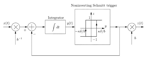
This paper shows that the circuit above can be implemented in real time and that {t_k} are sufficient to reconstruct x(t). The recovery algorithm looks pretty simple — multiplication by a certain pseudoinverse matrix. The second part of the paper deals with the stability of the system with respect to errors in the decoder parameter or time quantization. The compare the scheme to irregular sampling algorithms. The tools they use for this analysis come from non-harmonic analysis, but the math isn’t all that rough.

This work is different than the sampling with a finite rate of innovation work of Vetterli, Marziliano, and Blu, which says (loosely) that regular sampling is good for a wider class of signals than bandlimited signals. It would be interesting to see if a TEM mechanism is good for those signals as well. That might be another robustness issue to explore.

Finally, one interesting connection (and possible another motivation for this work) is that neurons may be doing this kind of time encoding all the time. The integrate-and-fire model of a neuron is, from a black-box perspective, converting an input signal into a sequence of times, just like a TEM.

paper a day : The Byzantine Generals Problem

Posted on January 7, 2008 by Anand Sarwate

It’s more like “paper when I feel like it,” but whatever. This is a classic systems paper on decentralized agreement. Because the result is pretty general, I think there is something that could be done to connect it to information-theoretic studies of multi-way communication or maybe key agreement. That’s a bit hand-waving though.

The Byzantine Generals Problem
Leslie Lamport, Robert Shostak, and Marshall Pease
ACM Transactions on Programming Languages and Systems
Vol. 4 No. 3, July 1982, pp. 382–401.

The basic problem is pretty simple. There are n total generals, some of whom may be disloyal. A commanding general must send an order to n-1 lieutenant generals such that (a) all loyal lieutenants follow the same order and (b) if the commander is loyal then all loyal lieutenants follow the order sent by the commander. The paper looks a oral messages, which are unsigned messages such that a disloyal general can send any possible message, as well as signed messages. I’ll just talk about the former. A protocol for solving this problem is an algorithm for each general to execute, at the end of which all generals make a decision based on the information they have received.

The first result is that satisfying both conditions is impossible with m traitors unless n > 3m. This is easiest to see in the case of three generals, where you can go through all the cases. To extend it to general n the insight is that if n = 3m then m disloyal generals can collude to force indecision at m other generals. It’s kind of like having a devil on one shoulder and an angel on the other. If they are equally strong you will not be able to make the right choice. This result can be extended to show that approximate agreement (in a certain sense) is also impossible.

On the more side, for n > 3m there is a spreading/flooding algorithm that satisfies the conditions. The commander sends a message, and then each lieutenant general acts as the commander in a smaller instance of the algorithm to send the command to the remaining generals. This rebroadcasting protocol, while wasteful, guarantees that the loyal generals will all do the same thing. This algorithm can be extended to the case where the communication structure is a graph with certain “nice” structural properties.

To me, the interesting part really is the converse, since it says something about symmetrizing the distribution. The same phenomenon occurs in the arbitrarily varying channel, where the capacity is zero if a jammer can simulate a valid codeword. In this analogy, the encoder is one group of m generals, the decoder another group of m, and the jammer is a coalition of m disloyal generals.

There’s also a nice bit where they lay the smack down: “This argument may appear convincing, but we strongly advise the reader to be very suspicious of such nonrigorous reasoning. Although this result is indeed correct, we have seen equally plausible “proofs” of invalid results. We know of no area in computer science or mathematics in which informal reasoning is more likely to lead to errors than in the study of this type of algorithm.”

paper a day : auctions where the seller can restrict the supply

Posted on April 27, 2007 by Anand Sarwate

Auctions of divisible goods with endogenous supply
K. Back and J.F. Zender
Economics Letters 73 (2001) 29–34

I’m working on a research problem that has some relationship to auction theory, so I’m trying to read up on some of the literature. I finally found this paper, which is more related to what I’m doing — an auction in which the amount of the divisible good is determined after the bidding. This is used in Treasury auctions in some countries, but is also a reasonable model for a kind of “middleman scenario” I think, where the seller is a middleman and uses the bids to purchase the good to be sold from a supplier.

In a uniform-price auction (where the bidders bid demand curves and the seller sets a price), equilibria exists where the bidders bid really low and then get the good for free. This can be arbitrarily bad for the seller. In a discriminatory-price auction (where the price bidders pay is kind of like an integral of their demand curve), this problem doesn’t happen, since bidders are interested in their entire demand curve. This is good for the seller.

But you can fix up a uniform price auction by letting the seller restrict the supply after the bids come in, This paper shows that in that case, the equilibria are better for the seller, and in fact the seller will not have to restrict the supply. So by retaining the right to restrict the supply, the situation is improved, but that right need not be exercised.

paper a day : approximating high-dimensional pdfs by low-dimensional ones

Posted on February 18, 2007 by Anand Sarwate

Asymptotically Optimal Approximation of Multidimensional pdf’s by Lower Dimensional pdf’s
Steven Kay
IEEE Transactions on Signal Processing, V. 55 No. 2, Feb. 2007, p. 725–729

The title kind of says it all. The main idea is that if you have a sufficient statistic, then you can create the true probability density function (pdf) of the data from the pdf of the sufficient statistic. However, if there is no sufficient statistic, you’re out of luck, and you’d like to create a low-dimensional pdf that somehow best captures the features you want from the data. This paper proves that a certain pdf created by a projection operation is optimal in that it minimizes the Kullback-Leibler (KL) divergence. Since the KL divergence dictates the error in many hypothesis tests, this projection operation is good in that decisions based on the projected pdf will be close to decisions based on the true pdf.

This is a correspondence item, so it’s short and sweet — equations are given for the projection and it is proved to minimize the KL divergence to the true distribution. Examples are given for cases in which sufficient statistics exist and do not exist, and an application to feature selection for discrimination is given. The benefit is that this theorem provides a way of choosing a “good” feature set based on the KL divergence, even when the true pdf is not known. This is done by estimating an expectation from the observed data (the performance then depends on the convergence speed of the empirical mean to the true mean, which should be exponentially fast in the number of data points).

The formulas are sometimes messy, but it looks like it could be a useful technique. I have this niggling feeling that a “bigger picture” view would be forthcoming from looking at information geometry/differential geometry viewpoint, but my fluency in those techniques is lacking at the moment.

Update: My laziness prevented me from putting up the link. Thanks, Cosma, for keeping me honest!

paper a day : last encounter routing with EASE

Posted on February 12, 2007 by Anand Sarwate

Locating Mobile Nodes with EASE : Learning Efficient Routes from Encounter Histories Alone
M. Grossglauser and M. Vetterli
IEEE/ACM Transactions on Networking, 14(3), p. 457- 469

This paper deals with last encounter routing (LER), a kind of protocol in which location information for nodes is essentially computed “on the fly” and there is no need to disseminate a location table and update it. They consider a grid toplogy (a torus, actually) on which nodes do a simple random walk. The walk time is much slower than the transmission time, so at any moment the topology is frozen with respect to a single packet transmission. Every node i maintains a table of pairs (P_ij, A_ij) for each other node j where P is its last known position and A is the age of that information. In the Exponential Age SEarch protocol (EASE) and GReedy EASE (GREASE), a packet keeps in its header an estimate of the position of its destination, and rewrites that information when it meets a node with a closer and more recent estimate. Because the location information and mobility processes are local, these schemes performs order-optimally (but with worse constants) to routing with location information, and with no overhead in the cost.

In particular, EASE computes a sequence of anchors for the packet, each one of has an exponentially closer estimate of the destination in both time and space. For example, each anchor could halve the distance to the destination as well as the age of that location estimate. This is similar in spirit to Kleinberg’s small world graphs paper, in which routing in a small world graph halves the distance, leading to a log(n) routing time, which comes from long hops counting the same as local hops. Here long hops cost more, so you still need n^1/2 hops. The paper comes with extensive simulation results to back up the analysis, which is nice.

What is nicer is the intuition given at the end:

Intuitively, mobility diffusion exploits three salient features of the node mobility processes: locality, mixing, and homogeneity…
Locality ensure[s] that aged information is still useful… Mixing of node trajectories ensures that position information diffuses around this destination node… Homogeneity ensure[s] that the location information spreads at least as fast as the destination moves.

The upshot is that location information is essentially free in an order sense, since the mobility process has enough memory to guarantee that suboptimal greedy decisions are not too suboptimal.

paper a day : power laws for white/gray matter ratios

Posted on December 18, 2006 by Anand Sarwate

I swear I’ll post more often starting soon — I just need to get back into the swing of things. In the meantime, here’s a short but fun paper.

A universal scaling law between gray matter and white matter of cerebral cortex
K. Zhang and T. Sejnowski
PNAS v.97 no. 10 (May 9, 2000)

This paper looks at the brain structure of mammals, and in particular the volumes of gray matter (cell bodies, dendrites, local connections) and white mattern (longer-range inter-area fibers). A plot of white matter vs. gray matter volumes showing different mammals, from a pygmy shrew to an elephant, show a really close linear fit on a log-log scale, with the best line having a slope of log(W)/log(G) = 1.23. This paper suggests that the exponent can be explained mathematically using two axioms. The first is that a piece of cortical area sends and receives ths same cross-sectional area of long-range fibers. The second more important axiom is that the geometry of the cortex is designed to minimize the average length of the long-distance fibers.

By using these heuristics, they argue that an exponent of 4/3 is “optimal” with respect to the second criterion. The difference of 0.10 can be explained by the fact that cortical thickness increases with the size of the animal, so they regressed cortical thickness vs. log(G) to get a thickness scaling of 0.10. It’s a pretty cute analysis, I thought, although it can’t really claim that minimum wiring is a principle in the brain so much as the way brains are is consistent with minimal wiring. Of course, I don’t even know how you would go about trying to prove the former statement — maybe this is why I feel more at home in mathematical engineering than I do in science…

paper a day : an LP inequality for concentration of measure

Posted on November 12, 2006 by Anand Sarwate

A Linear Programming Inequality with Applications to Concentration of Measure
Leonid Kontorovich
ArXiV: math.FA/0610712

The name “linear programming” is a bit of a misnomer –it’s not that Kontorovich comes up with a linear program whose solution is a bound, but more that the inequality relates two different norms, and the calculation of one of them can be thought of as maximizing an inner product over a convex polytope, which can be solved as a linear program. This norm inequality is the central fact in the paper. There are two weighted norms on functions at work — one is defined via a recursion that looks a lot like the sum of martingale differences. The other is maximizing the inner product of the given function with functions in a polytope defined by the weights. All functions in the polytope have bounded Lipschitz coefficient. By upper bounding the latter norm with the former, he can apply the former to the Azuma/Hoeffding/McDiarmid inequalities that show measure concentration for functions with bounded Lipschitz coefficient.

On a more basic level, consider a function of many random variables. For example, the empirical mean is such a function. A bounded Lipschitz coefficient means they are “insensitive” to fluctuations in one value. This intuitively means that as we add more variables the function will not deviate from is mean value by very much. To show this, you need to bound a probability with the Lipschitz coefficient, which is exactly what this inequality is doing. Kontorovitch thereby obtains a generalization of the standard inequalities.

What I’m not sure about is how I would ever use this result, but that’s my problem, really. The nice thing about the paper is that it’s short, sweet, and to the point without being terse. That’s always a plus when you’re trying to learn something.

	Zonghong Liu on A story about Canvas
	anonymousskimmer on “The needs of the many,…
	Chanterelle Recipes… on Broiled shrimp with chanterell…
	kvarsh on ICML 2019 encouraged code subm…
	Pulkit Grover on gender inclusivity in communic…

An Ergodic Walk

a process whose average over time converges to the true average

Tag Archives: paper a day