UCI Repository Citation Change

Posted on July 26, 2013 by Anand Sarwate

When making an editing pass over a bibliography today, I noticed that the citation for the UC Irvine Machine Learning Repository has changed. It used to be
@misc{Bache+Lichman:2013 , author = "A. Asuncion and D.H. Newman", year = "2007", title = "{UCI} Machine Learning Repository", url = "http://archive.ics.uci.edu/ml", institution = "University of California, Irvine, School of Information and Computer Sciences" }
But now it’s this:
@misc{Bache+Lichman:2013 , author = "K. Bache and M. Lichman", year = "2013", title = "{UCI} Machine Learning Repository", url = "http://archive.ics.uci.edu/ml", institution = "University of California, Irvine, School of Information and Computer Sciences" }
Also, the KDD repository has been merged in with the main repository, so the above is now the citation for both.

Update your BibTeX accordingly! (You too Kunal, but I bet you don’t cite this repo that much).

ISIT Blogging, part 1

Posted on July 24, 2013 by Anand Sarwate

Here are my much-belated post-ISIT notes. I didn’t do as good a job of taking notes this year, so my points may be a bit cursory. Also, the offer for guest posts is still open! On a related note the slides from the plenary lectures are now available on Dropbox, and are also linked to from the ISIT website.

From compression to compressed sensing
Shirin Jalali (New York University, USA); Arian Maleki (Rice University, USA)
The title says it, mostly. Both data compression and compressed sensing use special structure in the signal to achieve a reduction in storage, but while all signals can be compressed (in a sense), not all signals can be compressively sensed. Can one get a characterization (with an algorithm) that can take a lossy source code/compression method, and use it to recover a signal via compressed sensing? They propose an algorithm called compressible signal pursuit to do that. The full version of the paper is on ArXiV.

Dynamic Joint Source-Channel Coding with Feedback
Tara Javidi (UCSD, USA); Andrea Goldsmith (Stanford University, USA)
This is a JSSC problem with a Markov source, which can be used to model a large range of problems, including some sequential search and learning problems (hence the importance of feedback). The main idea is to map the problem in to a partially-observable Markov decision problem (POMDP) and exploit the structure of the resulting dynamic program. They get some structural properties of the solution (e.g. what are the sufficient statistics), but there are a lot of interesting further questions to investigate. I usually have a hard time seeing the difference between finite and infinite horizon formulations, but here the difference was somehow easier for me to understand — in the infinite horizon case, however, the solution is somewhat difficult to compute.

Unsupervised Learning and Universal Communication
Vinith Misra (Stanford University, USA); Tsachy Weissman (Stanford University, USA)
This paper was about universal decoding, sort of. THe idea is that the decoder doesn’t know the codebook but it knows the encoder is using a random block code. However, it doesn’t know the rate, even. The question is really what can one say in this setting? For example, symmetry dictates that the actual message label will be impossible to determine, so the error criterion has to be adjusted accordingly. The decoding strategy that they propose is a partition of the output space (or “clustering”) followed by a labeling. They claim this is a model for clustering through an information theoretic lens, but since the number of clusters is exponential in the dimension of the space, I think that it’s perhaps more of a special case of clustering. A key concept in their development is something they call the minimum partition information, which takes the place of the maximum mutual information (MMI) used in universal decoding (c.f. Csiszár and Körner).

On AVCs with Quadratic Constraints
Farzin Haddadpour (Sharif University of Technology, Iran); Mahdi Jafari Siavoshani (The Chinese University of Hong Kong, Hong Kong); Mayank Bakshi (The Chinese University of Hong Kong, Hong Kong); Sidharth Jaggi (Chinese University of Hong Kong, Hong Kong)
Of course I had to go to this paper, since it was on AVCs. The main result is that if one considers maximal error but allow the encoder only to randomize, then one can achieve the same rates over the Gaussian AVC as one can with average error and no randomization. That is, allowing encoder randomization can move from average error to max error. An analogous result for discrete channels is in a classic paper by Csiszár and Narayan, and this is the Gaussian analogue. The proof uses a similar quantization/epsilon-net plus union bound that I used in my first ISIT paper (also on Gaussian AVCs, and finally on ArXiV), but it seems that the amount of encoder randomization needed here is more than the amount of common randomness used in my paper.

Coding with Encoding Uncertainty
Jad Hachem (University of California, Los Angeles, USA); I-Hsiang Wang (EPFL, Switzerland); Christina Fragouli (EPFL, Switzerland); Suhas Diggavi (University of California Los Angeles, USA)
This paper was on graph-based codes where the encoder makes errors, but the channel is ideal and the decoder makes no errors. That is, given a generator matrix $G$ for a code, the encoder wiring could be messed up and bits could be flipped or erased when parities are being computed. The resulting error model can’t just be folded into the channel. Furthermore, a small amount of error in the encoder (in just the right place) could be catastrophic. They focus just on edge erasures in this problem and derive a new distance metric between codewords that helps them characterize the maximum number of erasures that an encoder can tolerate. They also look at a random erasure model.

a cute paper: finding a most biased coin with fewest flips

Posted on July 19, 2013 by Anand Sarwate

I saw this paper on ArXiV a while back and figured it would be a fun read, and it was. Post-ISIT blogging may have to wait for another day or two.

Finding a most biased coin with fewest flips
Karthekeyan Chandrasekaran, Richard Karp
arXiv:1202.3639 [cs.DS]

The setup of the problem is that you have $n$ coins with biases $\{p_i : i \in [n]\}$ . For some given $p \in [\epsilon,1-\epsilon]$ and $\epsilon \in (0,1/2)$ , each coin is “heavy” ( $p_i = p + \epsilon$ ) with probability $\alpha$ and “light” ( $p_i = p - \epsilon$ ) with probability $1 - \alpha$ . The goal is to use a sequential flipping strategy to find a heavy coin with probability at least $1 - \delta$ .

Any such procedure has three components, really. First, you have to keep track of some statistics for each coin $i$ . On the basis of that, you need a rule to pick which coin to flip. Finally, you need a stopping criterion.

The algorithm they propose is a simple likelihood-based scheme. If I have flipped a particular coin $i$ a bunch of times and gotten $h_i$ heads and $t_i$ tails, then the likelihood ratio is
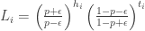
$L_i = \left( \frac{p+\epsilon}{p - \epsilon} \right)^{h_i} \left( \frac{ 1 - p - \epsilon }{ 1 -p + \epsilon} \right)^{t_i}$
So what the algorithm does is keep track of these likelihoods for the coins that it has flipped so far. But what coin to pick? It is greedy and chooses a coin $i$ which has the largest likelihood $L_i$ so far (breaking ties arbitrarily).

Note that up to now the prior probability $\alpha$ of a coin being heavy has not been used at all, nor has the failure probability $\delta$ . These appear in the stopping criterion. The algorithm keeps flipping coins until there exists at least one $i$ for which
$L_i \ge \frac{1 - \alpha}{\alpha} \cdot \frac{ 1 - \delta }{\delta}$
It then outputs the coin with the largest likelihood. It’s a pretty quick calculation to see that given $(h_i, t_i)$ heads and tails for a coin $i$,
$\mathbb{P}(\mathrm{coin\ }i\mathrm{\ is\ heavy}) = \frac{\alpha L_i}{ \alpha L_i + (1 - \alpha) }$ ,
from which the threshold condition follows.

This is a simple-sounding procedure, but to analyze it they make a connection to something called a “multitoken Markov game” which models the corresponding mutli-armed bandit problem. What they show is that for the simpler case given by this problem, the corresponding algorithm is, in fact optimal in the sense that it makes the minimum expected number of flips:
$\frac{16}{\epsilon^2} \left( \frac{1 - \alpha}{\alpha} + \log\left( \frac{(1 -\alpha)(1 - \delta)}{\alpha \delta} \right) \right)$

The interesting thing here is that the prior distribution on the heavy/lightness plays a pretty crucial role here in designing the algorithm. part of the explore-exploit tradeoff in bandit problems is the issue of hedging against uncertainty in the distribution of payoffs — if instead you have a good handle on what to expect in terms of how the payoffs of the arms should vary, you get a much more tractable problem.

Yet more skims from ArXiV

Posted on June 10, 2013 by Anand Sarwate

I’m still catching up on my backlog of ~~reading~~ everything, but I’ve decided to set some time aside to take a look at a few papers from ArXiV.

Lecture Notes on Free Probability by Vladislav Kargin, which is 100 pages of notes from a course at Stanford. Pretty self-explanatory, except for the part where I don’t really know free probability. Maybe reading these will help.
Capturing the Drunk Robber on a Graph by Natasha Komarov and Peter Winkler. This is on a simple pursuit-evasion game in which the robber (evader) is moving according to a random walk. On a graph with $n$ vertices:

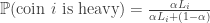the drunk will be caught with probability one, even by a cop who oscillates on an edge, or moves about randomly; indeed, by any cop who isn’t actively trying to lose. The only issue is: how long does it take? The lazy cop will win in expected time at most $4 n^3/27$ (plus lower-order terms), since that is the maximum possible expected hitting time for a random walk on an n-vertex graph [2]; the same bound applies to the random cop [4]. It is easy to see that the greedy cop who merely moves toward the drunk at every step can achieve $O(n^2)$ ; in fact, we will show that the greedy cop cannot in general do better. Our smart cop, however, gets her man in expected time $n + o(n)$ .

How do you make a smarter cop? In this model the cop can tell where the robber is but has to get there by walking along the graph. Strategies which try to constantly “retarget” are wasteful, so they propose a strategy wherein the cop periodically retargets to eventually meet the robber. I feel like there is a prediction/learning algorithm or idea embedded in here as well.
Normalized online learning by Stephane Ross, Paul Mineiro, John Langford. Normalization and data pre-processing is the source of many errors and frustrations in machine learning practice. When features are not normalized with respect to each other, procedures like gradient descent can behave poorly. This paper looks at dealing with data normalization in the algorithm itself, making it “unit free” in a sense. It’s the same kind of weights-update rule that we see in online learning but with a few lines changed. They do an adversarial analysis of the algorithm where the adversary gets to scale the features before the learning algorithm gets the data point. In particular, the adversary gets to choose the covariance of the data.
On the Optimality of Treating Interference as Noise, by Chunhua Geng, Navid Naderializadeh, A. Salman Avestimehr, and Syed A. Jafar. Suppose I have a $K$ -user interference channel with gains $\alpha_{ij}$ between transmitter $i$ and receiver $j$ . Then if
$\alpha_{ii} \ge \max_{j \ne i} \alpha_{ij} + \max_{k \ne i} \alpha_{ki}$
then treating interference as noise is optimal in terms of generalized degrees of freedom. I don’t really work on this kind of thing, but it’s so appealing from a sense of symmetry.
Online Learning under Delayed Feedback, byPooria Joulani, András György, Csaba Szepesvári. This paper is on forecasting algorithms which receive the feedback (e.g. the error) with a delay. Since I’ve been interested in communication with delayed feedback, this seems like a natural learning analogue. They provide ways of modifying existing algorithms to work with delayed feedback — one such method is to run a bunch of predictors in parallel and update them as the feedback is returned. They also propose methods which use partial monitoring and an approach to UCB for bandit problems in the delayed feedback setting.

MNIST error rates for SVM on projected data

Posted on May 20, 2013 by Anand Sarwate

I’ve started doing more machine learning research lately, which means I’ve been ~~sullying my delicate theorist’s hands~~ testing out my algorithms on data. Perhaps the most (over) used dataset is the MNIST handwritten digits collection, which was been put into MATLAB form by Sam Roweis (RIP). As a baseline, I wanted to see how an SVM would perform after I projected the data (using PCA) into the top 100 dimensions. The primal program is

$\min_{\mathbf{w},b} \frac{1}{2} \| \mathbf{w} \|_2^2 + C \sum_{i=1}^{n} z_i$
s.t. $y_i (\mathbf{w}^T \mathbf{x}_i + b) \ge 1 - z_i)$

I chose some “reasonable” value for C and tried to train a classifier on all pairs of points and got the following error rates on the test set (in percentages, rounded).

0
0      0
0.56   0.43   0
0.33   0.45   2.37   0
0.04   0.06   1.17   0.23   0
1.02   0.11   1.89   3.77   0.72   0
0.52   0      1.31   0.08   0.60   1.66   0
0.01   0.15   1.01   0.80   0.80   0.42   0      0
0.43   1.15   2.22   2.69   0.38   3.41   0.54   0.47   0 
0.20   0.14   0.85   1.13   3.03   1.02   0      3.82   1.27   0

This is digits from 0 to 9, so for example, the training error for classifying 0 versus 1 was zero percent, but it’s about 3.8 percent error to decide between 9 and 7. I did this to try and get a sense of which digits were “harder” for SVM to distinguish between so that I could pick a good pair for experiments, or better yet, to pick a pair based on a target error criterion. Running experiments on Gaussian synthetic examples is all fine and good, but it helps to have a range of data sets to test out how resilient an algorithm is to more noise, for example.

More ArXiV skims

Posted on April 23, 2013 by Anand Sarwate

Assumptionless consistency of the Lasso
Sourav Chatterjee
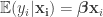The title says it all. Given $p$ -dimensional data points $\{ \mathbf{x}_i : i \in [n] \}$ the Lasso tries to fit the model $\mathbb{E}( y_i | \mathbf{x_i}) = \boldsymbol{\beta} \mathbf{x}_i$ by minimizing the $\ell^1$ penalized squared error
$\sum_{i=1}^{n} (y_i - \boldsymbol{\beta} \mathbf{x}_i)^2 + \lambda \| \boldsymbol{\beta} \|_1$ .
The paper analyzes the Lasso in the setting where the data are random, so there are $n$ i.i.d. copies of a pair of random variables $(\mathbf{X},Y)$ so the data is $\{(\mathbf{X}_i, Y_i) : i \in [n] \}$ . The assumptions are on the random variables $(\mathbf{X},Y)$ : (1) each coordinate $|X_i| \le M$ is bounded, the variable $Y = (\boldsymbol{\beta}^*)^T \mathbf{X} + \varepsilon$ , and $\varepsilon \sim \mathcal{N}(0,\sigma^2)$ , where $\boldsymbol{\beta}^*$ and $\sigma$ are unknown constants. Basically that’s all that’s needed — given a bound on $\|\boldsymbol{\beta}\|_1$ , he derives a bound on the mean-squared prediction error.

On Learnability, Complexity and Stability
Silvia Villa, Lorenzo Rosasco, Tomaso Poggio
This is a handy survey on the three topics in the title. It’s only 10 pages long, so it’s a nice fast read.

Adaptivity of averaged stochastic gradient descent to local strong convexity for logistic regression
Francis Bach
A central challenge in stochastic optimization is understanding when the convergence rate of the excess loss, which is usually $O(1/\sqrt{n})$ , can be improved to $O(1/n)$ . Most often this involves additional assumptions on the loss functions (which can sometimes get a bit baroque and hard to check). This paper considers constant step-size algorithms but where instead they consider the averaged iterate $\latex \bar{\theta}_n = \sum_{k=0}^{n-1} \theta_k$. I’m trying to slot this in with other things I know about stochastic optimization still, but it’s definitely worth a skim if you’re interested in the topic.

On Differentially Private Filtering for Event Streams
Jerome Le Ny
Jerome Le Ny has been putting differential privacy into signal processing and control contexts for the past year, and this is another paper in that line of work. This is important because we’re still trying to understand how time-series data can be handled in the differential privacy setting. This paper looks at “event streams” which are discrete-valued continuous-time signals (think of count processes), and the problem is to design a differentially private filtering system for such signals.

Gossips and Prejudices: Ergodic Randomized Dynamics in Social Networks
Paolo Frasca, Chiara Ravazzi, Roberto Tempo, Hideaki Ishii
This appears to be a gossip version of Acemoglu et al.’s work on “stubborn” agents in the consensus setting. They show similar qualitative behavior — opinions fluctuate but their average over time converges (the process is ergodic). This version of the paper has more of a tutorial feel to it, so the results are a bit easier to parse.

Expected number of faces in Gaussian polytopes

Posted on April 22, 2013 by Anand Sarwate

Last week I was reading Active Learning via Perfect Selective Classification by El-Yaniv and Wiener, and came across a neat result due to Hug and Reitzner that they use in some of their bounds for active learning on Gaussian distributions.

The setup is the following : let $X_1, X_2, \ldots, X_n$ be $n$ jointly Gaussian vectors with distribution $\mathcal{N}(0,I_d)$ in $\mathbb{R}^d$ . The convex hull $P_n$ of these points is called a Gaussian polytope. This is a random polytope of course, and we can ask various things about their shape : what is the distribution of the number of vertices, or the number of $k$ -faces? Let $f_k(P_n)$ be the number of $k$ -faces Distributions are hard, but for general $k$ the expected number of faces (as $n \to infty$ ) is given by

$\mathbb{E}[ f_k(P_n)] = \frac{2^d}{\sqrt{d}} \binom{d}{k+1} \beta_{k,d-1}(\pi \ln n)^{(d-1)/2} (1 + o(1))$ ,

where $\beta_{k,d-1}$ is the internal angle of a regular $(d-1)$ -simplex at one of its $k$ -dimensional faces. What Hug and Reitzner show is a bound on the variance (which then El-Yaniv and Plan use in a Chebyshev bound) : there exists a constant $c_d$ such that

$\mathrm{Var}( F_k(P_n) ) \le c_d (\ln n)^{(d-1)/2}$

So the variance of the number of $k$ -faces can be upper bounded by something that does not depend at all on the actual value of $k$ . In fact, they show that

$f_k(P_n) (\ln n)^{-(d-1)/2} \to \frac{2^d}{\sqrt{d}} \binom{d}{k+1} \beta_{k,d-1} \pi^{(d-1)/2}$

in probability as $n \to \infty$ . That is, appropriately normalized, the number of faces converges to a constant.

To me this result was initially surprising, but after some more thought it makes a bit more sense. If you give me a cloud of Gaussian points, then I need $k+1$ points to define a $k$ -face. The formula for the mean says that if I chose a random set of $k+1$ points, then approximately $\frac{2^d}{\sqrt{d}} \beta_{k,d-1}(\pi \ln n)^{(d-1)/2}$ fraction of them will form a real $k$ -face of the polytope. This also explains why the simplex-related quantity appears — points that are on “opposite sides” of the sphere (the level sets of the density) are not going to form a face together. As $n \to \infty$ this fraction will change, but effectively the rate of growth in the number of faces with $n$ is $(\ln n)^{(d-1)/2}$ , regardless of $k$ .

I’m not sure where this result will be useful for me (yet!) but it seemed like something that the technically-minded readers of the blog would find interesting as well.

ICML Workshop on Machine Learning with Test-Time Budgets

Posted on March 27, 2013 by Anand Sarwate

Venkatesh Saligrama sent out a call for an ICML workshop he is organizing:

I wanted to bring to your attention an ICML workshop on “Machine Learning with Test-Time Budgets” that I am helping organize. The workshop will be held during the ICML week. The workshop will feature presentations both from data-driven as well as model-based perspectives and will feature researchers from machine learning and control/decision theory.

We are accepting papers related to these topics. Please let me know if you have questions about the workshop or wish to submit a paper.

Bellairs Workshop 2013

Posted on February 23, 2013 by Anand Sarwate

I just wanted to write a few words about the workshop at the Bellairs Research Institute. I just returned from sunny Barbados to frigid Chicago, so writing this will help me remember the sunshine and sand:

The beach at Bathsheba on the east coast of Barbados

Mike Rabbat put on a great program this year, and there were lots of talks on a range of topics in machine learning, signal processing, and optimization. The format of the workshop was to have talks with lots of room for questions and discussion. Talks were given out on the balcony where we were staying, and we had to end at about 2:30 because the sunshine would creep into our conference area, baking those of us sitting too far west.

Continue reading →

ITA 2013 : part the third