One of the things I’m always asked when giving a talk on differential privacy is “how should we interpret  ?” There a lot of ways of answering this but one way that seems to make more sense to people who actually think about risk, hypothesis testing, and prediction error is through the “area under the curve” metric, or AUC. This post came out of a discussion from a talk I gave recently at Boston University, and I’d like to thank Clem Karl for the more detailed questioning.
For the purposes of this post, a randomized algorithm  is -differentially private if

for all pairs of data sets  and
and  containing
  individuals and differing in a single individual, and all measurable sets
  .
.
For cases where the output of has a density, we can interpret this as saying the log-likelihood ratio for the output of the distribution is bounded by :
 .
.
For those familiar with hypothesis testing, this guarantee is saying something about the hypothesis test between  and
and  being “hard.” One interpretation of differential privacy is that an adversary observing the output of the algorithm will have a difficult time inferring if the data of individual is
  or
or  , even if they know all
  other data points.
Wasserman and Zhou showed that the parameter controls power of this hypothesis test. Oh and Viswanath write this more explicitly as a pair of inequalities governing the tradeoff between the false-alarm and missed-detection probabilities:

 .
.
If we plot these against each other we get a picture like this:
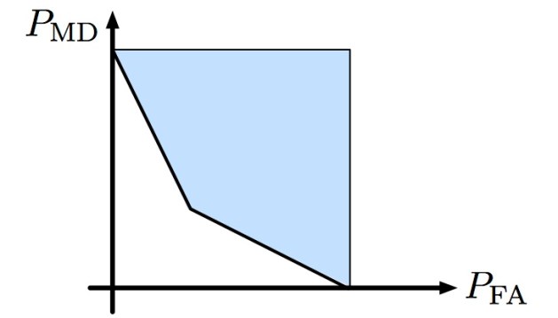
Probability of missed detection vs. probability of false alarm
The receiver operating characteristic (ROC) is defined as the true positive rate as a function of the false positive rate. That is, it’s  on the y-axis and
  on the x-axis. So this is the same plot as above, only flipped along the y-axis. To calculate the AUC we just integrate. The point where equality holds in both of the above inequalities is where
  , or
, or
 .
.
That’s the “corner point” in the previous figure. So the AUC is just
 .
.
We can plot the AUC as a function of pretty easily:

AUC versus epsilon for differential privacy
So we can now see how the privacy parameter affects the AUC for this hypothesis test. Depending on how comfortable you are with the risk (and also the threat model), you can assess for yourself what kind of you would prefer. Oh and Viswanath also calculate the tradeoff for  -differential privacy, but maybe I’ll leave that for another post. In the end, I don’t find this AUC plot so illuminating, but then again, I don’t have a visceral “feel” for how the AUC corresponds to the quality of the prediction.


