I owe Lav a response about birthdays, but in lieu of that, here are some links.
Via Matt Pugh, a grad student here, when intuition and math probably look wrong.
Via my father, what poetry and mathematics have in common.
I owe Lav a response about birthdays, but in lieu of that, here are some links.
Via Matt Pugh, a grad student here, when intuition and math probably look wrong.
Via my father, what poetry and mathematics have in common.
I think I lack the willpower to write up more notes on talks, and there are other things I’d like to blog about, but here are one or two sentences on some other talks that I found interesting… I also enjoyed the energy session on Friday and the talks by Sundeep and Galen on compressed sensing, but time has gotten the better of me. Next time, folks.
Channel Intrinsic Randomness
Matthieu Bloch
This was on extracting random bits from the output of noisy channel. These bits should be independent of the input to the channel. Matthieu uses the enigmatic information spectrum method to get his results — thanks to the plenary lecture I was able to understand it a bit better than I might have otherwise.
Assisted Common Information
Vinod Prabhakaran and Manoj Prabhakaran
I was very interested in this talk because I have been thinking of a related problem. Two terminals observe correlated sources 


Patterns and Exchangeability
N. P. Santhanam and M. Madiman
This work grew out of the AIM workshop on permanents. De Finetti’s theorem says an exchangeable process can be built up as a mixture of iid processes. Kingman showed that something called an exchangeable partition process is built up from something he called “paintbox processes.” One thing that we discovered at the workshop was that the pattern process of an iid process is the same as a paintbox process (and vice-versa). The paper then goes through many connections between these processes, certain limits of graphs, and connections to universal compression.
Universal Hypothesis Testing in the Learning-Limited Regime
Benjamin G. Kelly, Thitidej Tularak, Aaron B. Wagner, and Pramod Viswanath
This was a really great talk. The problem here is that for each 


Feature Extraction for Universal Hypothesis Testing via Rank-Constrained Optimization
Dayu Huang and Sean Meyn
This talk was of interest to me because I have been looking at hypothesis testing problems in connection with election auditing. In universal testing you know a lot about the distribution for one hypothesis, but much less about the other hypothesis. The Hoeffding test is a threshold test on the KL-divergence between the empirical distribution and the known hypothesis. This test is asymptotically optimal but has a high variance when the data is in high dimension. Thus for smaller sample sizes, a so-called mismatched divergence test may be better. In this paper they look at how to tradeoff the variance and the error exponent of the test.
I seem to have gotten all behind on wrapping up the ISIT blogging, so the remainder may be more compressed takes on things. This is not in the compressed sensing world, where the signals are sparse and my comments are meant to reconstruct, but more like lossy compression where 
Abbas El Gamal gave a very nice plenary on “Coding for Noisy Networks” in which he really brought together a lot of different eras and streams of work on network information theory and tried to tie them together in a conceptual framework. There was a nice mix of older and newer results. The thing I liked best about it was that he was very optimistic about making progress in understanding how to communicate in networks from an information-theory perspective, which counteracts the sentiment that I heard that “well, it’s just too messy.”
Te Sun Han gave the Shannon Lecture, of course, and he used his time to give a tutorial on the information spectrum method. I had tried to read the book earlier, and honestly found it a little impenetrable (or rather, I wasn’t sure what I was supposed to use from it). The talk was more like reading the papers — concisely stated, but with a clear line of intuition. I know some people are not a big fan of Shannon Lectures as tutorials, but I think there is also a case to be made that most people are unfamiliar with the information spectrum method. A nice example he gave was to show when the output of an optimal source coder looks “completely random.” Maybe this has been done already, but is there a connection between existing theories of pseudorandomness and the information spectrum method?
Cosma has posted a short proof of an ergodic theorem, which makes for some light weekend reading…
The remaining blogging from ISIT on my end will probably be delayed a bit longer since I have camera deadlines for EVT and ITW, a paper with Can Aysal for the special SP gossip issue that is within epsilon of getting done (and hence keeps getting put off) and a paper for Allerton with Michele Wigger and Young-Han Kim that needs some TLC. Phew! Maybe Alex will pick up the slack… (hint, hint)
Asynchronous Capacity per Unit Cost (Venkat Chandar, Aslan Tchamkerten, David Tse)
This paper was the lone non-adversarial coding paper in the session my paper was in. Aslan talked about a model for coding in which you have a large time block ![[0,A]](https://s0.wp.com/latex.php?latex=%5B0%2CA%5D&bg=ffffff&fg=333333&s=0&c=20201002)


Moderate Deviation Analysis of Channel Coding: Discrete Memoryless Case (Yucel Altug, Aaron Wagner)
This was a paper that looked at a kind of intermediate behavior in summing and normalizing random variables. If you sum up 

where 


Minimum energy to send k bits with and without feedback (Yury Polyanskiy, H. Vincent Poor, Sergio Verdu)
This was on the energy to send a bit but in the non-asymptotic energy regime (keeping philosophically with the earlier line of work by the authors) for the AWGN channel. Without feedback they show an achievability and converse for sending 


For many of the talks I attended I didn’t take notes — partly this is because I didn’t feel expert enough to note things down correctly, and partly because I am
RÉNYI DIVERGENCE AND MAJORIZATION (Tim van Erven; Centrum Wiskunde & Informatica, Peter Harremoës; Copenhagen Business College)
Peter gave a talk on some properties of the Rényi entropy
where 


MINIMAX LOWER BOUNDS VIA F-DIVERGENCES (Adityanand Guntuboyina; Yale University)
This talk was on minimax lower bounds on parameter estimation which can be calculated in terms of generalized
Suppose 


This has a very geometric feel to it but I had a bit of a hard time following all of the material since I didn’t know the related literature very well (much of it was given in relation to Yang and Barron’s 1999 paper).
MUTUAL INFORMATION SADDLE POINTS IN CHANNELS OF EXPONENTIAL FAMILY TYPE (Todd Coleman; University of Illinois, Maxim Raginsky; Duke University)
In some cases where we have a class of channels and a class of channel inputs, there is a saddle point. The main example is that Gaussian noise is the worst for a given power constraint and Gaussian inputs are the best. Another example is the “bits through queues” This paper gave a more general class of channels of “exponential family type” and gave a more general condition under which you get a saddle point for the mutual information. The channel models are related to Gibbs variational principle, and the arguments had a kind of “free energy” interpretation. Ah, statistical physics rears its head again.
INFORMATION-THEORETIC BOUNDS ON MODEL SELECTION FOR GAUSSIAN MARKOV RANDOM FIELDS (Wei Wang, Martin J. Wainwright, Kannan Ramchandran; University of California, Berkeley)
This was on two problems: inferring edges in a graphical model from iid samples from that model, and inverse covariance estimation. They are similar, but not quite the same. The goal was to prove necessary conditions for doing this; these necessary conditions match the corresponding achievable rates from polytime algorithms. The main result was that you need 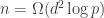


Perhaps malapropos for the NBA Finals, Prof. Michael Jordan gave the first plenary talk at ISIT. It was a great overview of nonparametric Bayesian modeling. In particular, he covered his favorite Chinese restaurant process (also known as the Pitman-Yor stick-breaking process), hierarchical Dirichlet priors, and all the other jargon-laden elements of modeling. At the end he covered some of the rather stunning successes of this approach in applications with lots of data to learn from. What was missing for me was a sense of how these approaches worked in the data-poor regime, so I asked a question (foolishly) about sample complexity. Alas, since that is a “frequentist” question and Jordan is a “Bayesian,” I didn’t quite get the answer to the question I was trying to ask, but that’s what happens when you don’t phrase things properly.
One nice thing that I learned was the connection to Kingman’s earlier work on characterizing random measures via non-homogeneous Poisson processes. Kingman has been popping up all over the place in my reading, from urn processes to exchangeable partition processes (also known as paintbox processes). When I get back to SD, it will be back to the classics for me!
Steven Strogatz has a column up on why it’s easier to think about natural frequencies rather than conditional probabilities.
A new postdoc here, Punyaslok Purkayastha, pointed out to me a Probability Surveys paper by Robin Pemantle on random processes with reinforcement, and I’ve been reading through it in spare moments (usually on the bus). I have had a problem knocking about my head that is related (Ram Rajagopal and I thought we could do in our spare time but we never managed to find enough time to work on it). All this stuff is pretty well-known already, but I thought it was a nice story.
A Polya urn process starts by taking an urn with 


To figure out the asymptotic behavior of this process, just note that the sequence of colors is exchangeable. If 

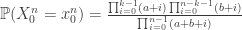
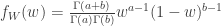
From this it is clear that the probability of seeing $x_1^n$ only depends on its type (empirical distribution, for non-information theorists). Since the sequence is exchangeable, de Finetti’s Theorem shows that the fraction of red balls 


A more general process is the Friedman urn process, in which you add 


Let’s look at a special case where instead of adding a ball of the same color that you drew, you only add a ball of the opposite color (which is a Friedman process with parameters (0,1)). Freedman’s result doesn’t apply here, but Kingman has a nice paper (which I am reading now) relating this process to a third process: the OK Corral process.
In the OK Corral process, say we start with 


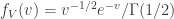
converges to a gamma distribution with parameter 1/2:
The weird thing about this is that the scaling is 
Kingman and Volkov extend the analysis by embedding the urns into birth processes, which is another technique for balls-into-bins with feedback of urns with reinforcement. But that’s another story for another time (but maybe not another blog post, this one took a bit longer than I expected).
One of the fun thing about graphical models is that arguments can be done by looking at diagrams (kind of like a diagram chase in algebraic topology). One such trick is from R.D. Shachter’s paper in UAI called “Bayes-Ball: The Rational Pastime (for Determining Irrelevance and Requisite Information in Belief Networks and Influence Diagrams)” (see it here. for example). This is a handy method for figuring out conditional independence relations, and is a good short-cut for figuring out when certain conditional mutual information quantities are equal to 0. The diagram below shows the different rules for when the ball can pass through a node or when it bounces off. Gray means that the variable is observed (or is in the conditioning). I tend to forget the rules, so I made this little chart summary to help myself out.