the MAP perturbation framework

I started working this fall on an interesting problem (shameless plug!) with Francesco Orabona, Tamir Hazan, and Tommi Jaakkola. What we do there is basically a measure concentration result, but I wanted to write a bit about the motivation for the paper. It’s nicely on the edge of that systems EE / CS divide, so I thought it might be a nice topic for the blog. One name for this idea is “MAP perturbations” so the first thing to do is explain what that means. The basic idea is to take a posterior probability distribution (derived from observed data) and do a random perturbation of the probabilities, and then take the maximum of that perturbed distribution. Sometimes this is called “perturb-and-MAP” but as someone put it, that sounds a bit like “hit-and-run.”

The basic problem is to sample from a particular joint distribution on n variables. For simplicity, let’s consider an n-bit vector \mathbf{x} \in \{0,1\}^n. There are 2^n possible values, so explicitly maximizing the distribution could be computationally tricky. However we are often aided by the fact probability model has some structure. For example, the n bits may be identified with labels {foreground,background} and correspond to n pixels in an image, and there may be some local constraints which make it more likely for adjacent pixels to have the same label. In general, these local constraints get lumped together into a potential function \theta(\mathbf{x}) which assigns a score to each \mathbf{x}. The distribution on \mathbf{x} is a Gibbs distribution:

p(\mathbf{x}) = \frac{1}{Z} \exp(\theta( \mathbf{x} ))

where the normalizing constant Z is the infamous partition function:

Z = \sum_{\mathbf{x}} \exp(\theta(\mathbf{x}))

It’s infamous because it’s often hard to compute explicitly. This also makes sampling from the Gibbs distribution hard.

The MAP rule chooses the \mathbf{x} that maximizes this distribution. Doing this means you don’t need to calculate Z since you can maximize the potential function instead:

\mathbf{X}_{\mathsf{MAP}} =  \mathrm{argmax} \left\{ \theta(\mathbf{x}) \right\}.

This isn’t any easier in general, computationally, but people have put lots of blood, sweat, and tears into creating MAP solvers that use tricks to do this maximization. In some cases, these solvers work pretty well. Our goal will be to use the good solvers as a black box.

Unfortunately, in a lot of applications, we really would like to sample from he Gibbs distribution, because the number-one best configuration \mathbf{x} may not be the only “good” one. In fact, there may be many almost-maxima, and sampling will let you produce a list of those. One way to do this is via Markov-chain Monte Carlo (MCMC), but the problem with all MCMC methods is you have to know how long to run the chain.

The MAP perturbation approach is different — it adds a random function \gamma(\mathbf{x}) to the potential function and solves the resulting MAP problem:

\mathbf{X}_{\mathsf{R-MAP}} =  \mathrm{argmax} \left\{ \theta(\mathbf{x}) + \gamma(\mathbf{x}) \right\}

The random function \gamma(\cdot) associates a random variable to each \mathbf{x}. The simplest approach to designing a perturbation function is to associate an independent and identically distributed (i.i.d.) random variable \gamma(\mathbf{x}) for each \mathbf{x}. We can find the distribution of the randomized MAP predictor when each \gamma(\mathbf{x}) a Gumbel random variable with zero mean, variance \pi^2/6, and cumulative distribution function

G( y ) = \exp( - \exp( - (y + c))),

where c \approx 0.5772 is the Euler-Mascheroni constant.

So what’s the distribution of the output of the randomized predictor \mathbf{X}_{\mathsf{R-MAP}}? It turns out that the distribution is exactly that of the Gibbs distribution we want to sample from:

\mathbb{P}_{\gamma}\left( \mathbf{X}_{\mathsf{R-MAP}} = \mathbf{x} \right) = p(\mathbf{x})

and the expected value of the maximal value is the log of the partition function:

\mathbb{E}_{\gamma}\left[ \max_{\mathbf{x}} \left\{ \theta(\mathbf{x}) + \gamma(\mathbf{x}) \right\} \right] = \log Z

This follows from properties of the Gumbel distribution.

Great – we’re done. We can just generate the \gamma random variables, shove the perturbed potential function into our black-box MAP solver, and voilà: samples from the Gibbs distribution. Except that there’s a little problem here – we have to generate 2^n Gumbel variables, one for each \mathbf{x}, so we’re still a bit sunk.

The trick is to come up with lower-complexity perturbation (something that Tamir and Tommi have been working on for a bit, among others), but I will leave that for another post…

expected time for an optimal game of memory

Via Dan Katz, I learned about a recent problem (warning: JSTOR) from the American Mathematical Monthly (a publication of the Mathematics Association of America, making shaded icosahedrons look cool for almost 100 years):

What to Expect in a Game of Memory
Author(s): Daniel J. Velleman, Gregory S. Warrington
The American Mathematical Monthly, Vol. 120, No. 9 (November), pp. 787-805

The game of memory is played with a deck of n pairs of cards. The cards in each pair are identical. The deck is shuffled and the cards laid face down. A move consists of flipping over first one card and then another. The cards are removed from play if they match. Otherwise, they are flipped back over and the next move commences. A game ends when all pairs have been matched. We determine that, when the game is played optimally, as n \rightarrow \infty
• The expected number of moves is (3 - 2 \ln 2) n + 7/8 - 2 \ln 2 \approx 1.61 n.
• The expected number of times two matching cards are unwittingly flipped over is \ln 2.
• The expected number of flips until two matching cards have been seen is 2^{2n} / \binom{2n}{n} \approx \sqrt{\pi n}.

This is not a competitive game of memory, but the singe player version. It’s a kind of explore-exploit tradeoff with a simple structure — if you know how to exploit, do it. Note that one could do 2 n moves by flipping every card over once (there are 2n cards) to learn all of their identities and then removing all of the pairs one by one. The better strategy is

  1. Remove any known pair.
  2. If no known pair is known, flip a random unknown card and match it if you can.
  3. If the first card is not matchable, flip another random unknown card to learn its value (and remove the pair if it matches.

This strategy exploits optimally when it can and explores optimally when it can’t. The second bullet point in the abstract is the gain from getting lucky, i.e. two randomly drawn cards matching.

The paper is an interesting read, but the arguments are all combinatorial. Since the argument is a limiting one as n \to \infty, I wonder if there is a more “probabilistic” argument (this is perhaps a bit fuzzy) for the results.

dismissing research communities is counterproductive

I recently saw that Andrew Gelman hasn’t really heard of compressed sensing. As someone in the signal processing/machine learning/information theory crowd, it’s a little flabbergasting, but I think it highlights two things that aren’t really appreciated by the systems EE/algorithms crowd: 1) statistics is a pretty big field, and 2) the gulf between much statistical practice and what is being done in SP/ML research is pretty wide.

The other aspect of this is a comment from one of his readers:

Meh. They proved L1 approximates L0 when design matrix is basically full rank. Now all sparsity stuff is sometimes called ‘compressed sensing’. Most of it seems to be linear interpolation, rebranded.

I find such dismissals disheartening — there is a temptation to say that every time another community picks up some models/tools from your community that they are reinventing the wheel. As a short-hand, it can be useful to say “oh yeah, this compressed sensing stuff is like the old sparsity stuff.” However, as a dismissal it’s just being parochial — you have to actually engage with the use of those models/tools. Gelman says it can lead to “better understanding one’s assumptions and goals,” but I think it’s more important to “understand what others’ goals.”

I could characterize rate-distortion theory as just calculating some large deviations rate functions. Dembo and Zeitouni list RD as an application of the LDP, but I don’t think they mean “meh, it’s rebranded LDP.” For compressed sensing, the goal is to do the inference in a computationally and statistically efficient way. One key ingredient is optimization. If you just dismiss all of compressed sensing as “rebranded sparsity” you’re missing the point entirely.

estimating probability metrics from samples

I took a look at this interesting paper by Sriperumbudur et al., On the empirical estimation of integral probability metrics (Electronic Journal of Statistics Vol. 6 (2012) pp.1550–1599). The goal of the paper is to estimate a distance or divergence between two distributions P and Q based on samples from each distribution. This sounds pretty vague at first… what kind of distributions? How many samples? This paper looks at integral probability metrics, which have the form

\gamma(P,Q) = \sup_{f \in \mathcal{F}} \left| \int_{S} f dP - \int_{S} f dQ \right|

where S is a measurable space on which P and Q are defined, and \mathcal{F} is a class of real-valued bounded measurable functions on S. This class doesn’t contain Csiszár \phi-divergences (also known as Ali-Silvey distances), but does contain the total variational distance.

Different choices of the function class give rise to different measures of difference used in so-called two-sample tests, such as the Kolmogorov-Smirnov test. The challenge in practically using these tests is that it’s hard to get bounds on how fast an estimator of \gamma(P,Q) converges if we have to estimate it from samples of P and Q. The main result of the paper is to provide estimators with consistency and convergence guarantees. In particular, they estimators are based on either linear programming or (in the case of kernel tests) in closed form.

The second section of the paper connects tests based on IPMs with the risk associated to classification rules for separating P and Q when the separation rule is restricted to come from the function class \mathcal{F} associated to the rule. This is a nice interpretation of these two-sample tests — they are actually doing similar things for restricted classes of classifiers/estimators.

Getting back to KL divergence and non-IPM measures, since total variation gives a lower bound on the KL divergence, they also provide lower bounds on the total variation distance in terms of other IPM metrics. This is important since the total variation distance can’t be estimated itself in a strongly consistent way. This could be useful for algorithms which need to estimate the total variation distance for continuous data. In general, estimating distances between multivariate continuous distributions can become a bit of a mess when you have to use real data — doing a plug-in estimate using, e.g. a kernel density estimator is not always the best way to go, and instead attacking the distance you want to measure directly could yield better results.

Bounds between common information and mutual information

I’m at EPFL right now on my way back from a trip to India. My last work-related stop there was the Tata Institute of Fundamental Research, where I am working with Vinod Prabhakaran on some follow-up work to our ISIT paper this year on correlated sampling. TIFR has a lovely campus in Navy Nagar, right next to the ocean in the south of Mumbai. It’s a short walk across the lawn to the ocean:

The beach at TIFR, looking north to the haze-obscured skyline of Mumbai

The beach at TIFR, looking north to the haze-obscured skyline of Mumbai

The grounds themselves are pretty rigorously landscaped and manicured:

The main building seen across the lawn in front of the ocean.

The main building seen across the lawn in front of the ocean.

Earlier in my trip I visited IIT-Madras, hosted by Andrew Thangaraj and Radha Krishna Ganti and IIT-Bombay, where I was working with Bikash Dey on extensions to some of our AVCs-with-delay work. It’s been a great trip and it’s nice to visit so many different schools. The challenges facing Indian higher education are very different than those in the US, and it’s a good change of perspective from my usual US-centric view of things. Maybe I’ll write more on that later.

But for now, I wanted to get back to some actual technical stuff, so I thought I’d mention something that came up in the course of my discussions with Vinod today. For a joint distribution P(X,Y), Wyner defined the common information in the the following way:

\mathsf{CI}(X;Y) = \min_{X--U--Y} I(XY ; U)

One fun fact about the common information is that it’s larger than the mutual information, so I(X;Y) \le \mathsf{CI}(X;Y)
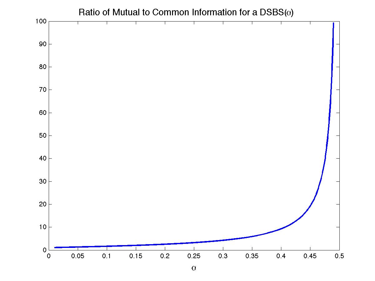
. One natural question that popped up as part of a calculation we had to do was whether for doubly-symmetric binary sources we could have a bound like

\mathsf{CI}(X;Y) \le \alpha I(X;Y)

for some “nice” \alpha. In particular, it would have been nice for us if the inequality held with \alpha = 2 but that turns out to not be the case.

Suppose (X,Y) and are a doubly-symmetric binary source, where Y is formed from X \sim \mathsf{Bern}(1/2) by passing it through a binary symmetric channel (BSC) with crossover probability \alpha. Clearly the mutual information is I(X;Y) = 1 - h(\alpha). For the common information, we turn to Wyner’s paper, which says \mathsf{CI}(X;Y) = 1 + h(\alpha) - 2 h( \frac{1}{2}( 1 - \sqrt{1 - 2 \alpha} ) ), which is a bit of a weird expression. Plotting the two for \alpha between 0 and 1/2 we get:

Mutual and Common Information for a DSBS

Mutual and Common Information for a DSBS

If we plot the ratio \mathsf{CI}(X;Y)/I(X;Y) versus \alpha, we get the following:

Ratio of Common to Mutual Information for a DSBS

Ratio of Common to Mutual Information for a DSBS


The ratio blows up! So not only is Common Information larger than mutual information, it can be an arbitrarily large factor larger than the mutual information.

It might seem like this is bad news for us, but it just made the problem we’re working on more interesting. If we get any results on that I might be less engimatic and blog about it.

Linkage

I am traveling all over India at the moment so I’m not really able to write contentful posts. Here are even more links instead, sigh. Maybe later I’ll talk about log-Sobolev inequalities so I can be cool like Max.

Speaking of Max, he posted this hilarious bad lip reading version of Game of Thrones. Probably NSFW. I don’t even like the series but it’s pretty funny.

For those who are fans of Rejected, Don Hertzfeldt’s new film is available on Vimeo.

Those who were at Berkeley may remember seeing Ed Reed perform at the Cheeseboard. His album (which I helped fund via indiegogo, was named a Downbeat Editors’ Pick. It’s a great album.

In light of the Snowden leaks, some doubt has been cast on NIST’s crypto standards.

I’m super late to this, but I endorse Andrew’s endorsement of Sergio‘s interview with Robert Fano in the IT Newsletter. Here’s just the article, if you want that.

GmailTeX

Avleen Bijral, one of the students here at TTIC, sent me a link to a pretty cool browser plugin for GMail called GMail TeX. Basically it lets you send LaTeX formatted emails via gmail. This can be quite a time saver for the reader (but maybe not the writer) if you’re remotely collaborating on some project (which I so often am these days, it seems). It’s supported on a wide variety of browsers and seems worth checking out!

PSA: immigration scams preying on international students

I got an email from the Rutgers ECE department about a new scam that has been preying on international students. Some readers of the blog may wish to be aware of this.

Scammers posing as immigration officials – United States Citizenship and Immigration Services (USCIS) officers, Department of State (DOS) officials, or local policemen are contacting international students, & scholars. They may ask for your personal information (such as SSN, passport number, credit card information), identify false problems with your immigration record, and ask for payment to correct the record.

These scams can be very sophisticated with a USCIS like number appearing on your caller ID, the caller knowing a lot of your personal information and so on. Here are a few pointers to bear in mind if you receive this kind of a fake “immigration” call:

  • Don’t wire/pay any money. USCIS will never call someone to ask for any form of payment over the phone.
  • Just hang up and don’t call back.
  • Call the real USCIS National Customer Service Center at 1-800-375-5283 to report the issue.
  • Never give out your personal information. No matter who a caller claims to be, don’t give him/her your I-94 number, “A” number, visa control number or any other personal information. Hang up and call the real USCIS.

Apparently Rutgers had an incident involving a postdoc, where the caller posed as a police officer “and informed the scholar that he had immigration problems. This female caller had the scholar’s home address, cell phone number and SSN number. She informed the scholar that the problem can be resolved if he could make an immediate payment.”

More information can be found at the USCIS website.

Postdoc at INRIA-ENS Paris on Graphs, Algorithms and Probability

Applications are invited for a Postdoc position (full-time, up to 2 years) at INRIA-ENS in Paris. The position is funded by the ANR GAP grant “Graphs, Algorithms and Probability.”

Requirements are a PhD degree in Computer Science or Mathematics and a strong background in some of the following topics:

  • discrete probability
  • statistical learning
  • combinatorial optimization
  • stochastic networks

Applications must include a research statement, a CV and the names and contacts of references. All material should be sent by email to Marc Lelarge. Please indicate in the subject POSTDOC GAP.

Important dates:

  • Intention of application (short email): as soon as possible
  • Deadline for application: December 1st, 2013
  • Suggested starting dates: Jan.-Feb. 2014

Linkage

A map of racial segregation in the US.

Vi Hart explains serial music (h/t Jim CaJacob).

More adventures in trolling scam journals with bogus papers (h/t my father).

Brighten does some number crunching on his research notebook.

Jerry takes “disruptive innovation” to task.

Vladimir Horowitz plays a concert at the Carter White House. Also Jim Lehrer looks very young. The program (as cribbed from YouTube)

  • The Star-Spangled Banner
  • Chopin: Sonata in B-flat minor, opus 35, n°2
  • Chopin: Waltz in a minor, opus 34, n°2
  • Chopin: Waltz in C-sharp minor, opus 64, n° 2
  • Chopin: Polonaise in A-flat major, opus 53 ,Héroïque
  • Schumann: Träumerei, Kinderszene n°7
  • Rachmaninoff: Polka de W.R
  • Horowitz: Variations on a theme from Bizet’s Carmen

The Simons Institute is going strong at Berkeley now. Moritz Hardt has some opinions about what CS theory should say about “big data,” and how it might be require some adjustments to ways of thinking. Suresh responds in part by pointing out some of the successes of the past.

John Holbo is reading Appiah and makes me want to read Appiah. My book queue is already a bit long though…

An important thing to realize about performance art that makes a splash is that it can be often exploitative.

Mimosa shows us what she sees.