Kamalika pointed me to this paper by Bin Yu in a Festschrift for Lucien Le Cam. People who read this blog who took information theory are undoubtedly familiar with Fano’s inequality, and those who are more on the CS theory side may have heard of Assouad (but not for this lemma). This paper describes the relationship between several lower bounds on hypothesis testing and parameter estimation.
Suppose we have a parametric family of distributions  , where
  is a metric space with metric
  . For two distributions
  and
and  define the affinity
  by:
by:

Let  denote the convex hull. Then Le Cam’s lemmas is the following.
Le Cam’s Lemma. Let  be an estimator of
  on
on  . Suppose
  and
and  be two sets such that
  for all
  , and
, and  and
and  be two subsets of such that
  when
when  . Then
![\sup_{P \in \mathcal{P}} \mathbb{E}_P[ d(\hat{\theta}, \theta(P)) ] \ge \delta \cdot \sup_{P_i \in \mathop{\rm co}(\mathcal{P}_i)} \| P_1 \wedge P_2 \|](https://s0.wp.com/latex.php?latex=%5Csup_%7BP+%5Cin+%5Cmathcal%7BP%7D%7D+%5Cmathbb%7BE%7D_P%5B+d%28%5Chat%7B%5Ctheta%7D%2C+%5Ctheta%28P%29%29+%5D+%5Cge+%5Cdelta+%5Ccdot+%5Csup_%7BP_i+%5Cin+%5Cmathop%7B%5Crm+co%7D%28%5Cmathcal%7BP%7D_i%29%7D+%5C%7C+P_1+%5Cwedge+P_2+%5C%7C&bg=ffffff&fg=333333&s=0&c=20201002)
This lemma gives a lower bound on the error of parameter estimates in terms of the total variational distance between the distributions associated to different parameter sets. It’s a bit different than the bounds we usually think of like Stein’s Lemma, and also a bit different than bounds like the Cramer-Rao bound.
Le Cam’s lemma can be used to prove Assouad’s lemma, which is a statement about a more structured set of distributions indexed by the  , the vertices of the hypercube. We’ll write
  for
for  if they differ in the j-th coordinate.
Assouad’s Lemma. Let  be a set of
  probability measures indexed by
  , and suppose there are
  pseudo-distances
  on such that for any pair

and that if

Then
![\max_{P_t \in \mathcal{F}_m} \mathbb{E}_{t}[ d(\hat{\theta},\theta(P_t))] \ge m \cdot \frac{\alpha_m}{2} \min\{ \|P_t \wedge P_{t'} \| : t \sim_j t', j \le m\}](https://s0.wp.com/latex.php?latex=%5Cmax_%7BP_t+%5Cin+%5Cmathcal%7BF%7D_m%7D+%5Cmathbb%7BE%7D_%7Bt%7D%5B+d%28%5Chat%7B%5Ctheta%7D%2C%5Ctheta%28P_t%29%29%5D+%5Cge+m+%5Ccdot+%5Cfrac%7B%5Calpha_m%7D%7B2%7D+%5Cmin%5C%7B+%5C%7CP_t+%5Cwedge+P_%7Bt%27%7D+%5C%7C+%3A+t+%5Csim_j+t%27%2C+j+%5Cle+m%5C%7D&bg=ffffff&fg=333333&s=0&c=20201002)
The min comes about because it is the weakest over all neighbors (that is, over all j) of  in the hypercube. Assouad’s Lemma has been used in various different places, from covariance estimation, learning, and other minimax problems.
Yu then shows how to prove Fano’s inequality from Assouad’s inequality. In information theory we see Fano’s Lemma as a statement about random variables and then it gets used in converse arguments for coding theorems to bound the entropy of the message set. Note that a decoder is really trying to do a multi-way hypothesis test, so we can think about the result in terms of hypothesis testing instead. This version can also be found in the Wikipedia article on Fano’s inequality.
Fano’s Lemma. Let  contain
  probability measures such that for all
  with
with 
and

Then
![\max_j \mathbb{E}_j[ d(\hat{\theta},\theta(P_j)) ] \ge \frac{\alpha_r}{2}\left( 1 - \frac{\beta_r + \log 2}{\log r} \right)](https://s0.wp.com/latex.php?latex=%5Cmax_j+%5Cmathbb%7BE%7D_j%5B+d%28%5Chat%7B%5Ctheta%7D%2C%5Ctheta%28P_j%29%29+%5D+%5Cge+%5Cfrac%7B%5Calpha_r%7D%7B2%7D%5Cleft%28+1+-+%5Cfrac%7B%5Cbeta_r+%2B+%5Clog+2%7D%7B%5Clog+r%7D+%5Cright%29&bg=ffffff&fg=333333&s=0&c=20201002)
Here  is the KL-divergence. The proof follows from the regular Fano’s inequality by choosing a message
  uniformly in
  and then setting the output
  to have the distribution
  conditioned on
  .
.
The rest of the paper is definitely worth reading, but to me it was nice to see that Fano’s inequality is interesting beyond coding theory, and is in fact just one of several kinds of lower bound for estimation error.

 that is
  , so zero-mean and unit variance. If I observe
  where
where  is also
![\mathbb{E}[ (S - \hat{S})^2 ] = 1/2](https://s0.wp.com/latex.php?latex=%5Cmathbb%7BE%7D%5B+%28S+-+%5Chat%7BS%7D%29%5E2+%5D+%3D+1%2F2&bg=ffffff&fg=333333&s=0&c=20201002) . The question is this: can we somehow get an MSE of less than 1/2 by “encoding”
. The question is this: can we somehow get an MSE of less than 1/2 by “encoding”  and let
  , and
, and  but with the restriction that
  . That is, the encoding cannot take any more power.
 iid unit variance Gaussians
  and you want to estimate
  where
where  is iid unit variance Gaussian as well. The goal is to minimize the average per-letter distortion:
![d(\hat{S}^n, S^n) = \frac{1}{n} \sum_{i=1}^{n} \mathbb{E}[ (S_i - \hat{S}_i)^2 ]](https://s0.wp.com/latex.php?latex=d%28%5Chat%7BS%7D%5En%2C+S%5En%29+%3D+%5Cfrac%7B1%7D%7Bn%7D+%5Csum_%7Bi%3D1%7D%5E%7Bn%7D+%5Cmathbb%7BE%7D%5B+%28S_i+-+%5Chat%7BS%7D_i%29%5E2+%5D&bg=ffffff&fg=333333&s=0&c=20201002)
 . Since separate source coding (compression) followed by channel coding (error control) is optimal, in order to get distortion
  the rate
  so
so  . Furthermore, this is achievable with no coding at all by just setting
  .
. grid with the top and left edges wrapped around to connect with the bottom and right edges. Every vertex has 4 neighbors. Now imagine a very lazy random walk on this graph in which a random walker moves from vertex
  to one of its neighbors with probability
  . It’s “well known” that this random walk takes around
  steps to mix. That is, if
  is the matrix of transition probabilities then
 is the second largest eigenvalue of
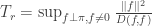
  is the inverse of the spectral gap of the matrix. One way of characterizing
  on the states of the chain define the Dirichlet form
  by
by
 and
and  for all edges in the graph. We write
  if
if
 via
via
 is divisible by 4 and set
  . The values for

 and
and  and there are fewer than
  . Thus:
 as desired.
 but in the denominator we get
  positive terms. The key is to make all the differences
  in the denominator small while keeping the average of
  large enough. Even though you sum over
  in the numerator.