Gaussian channel capacity and angles

There’s this nice calculation in a paper of Shannon’s on optimal codes for Gaussian channels which essentially provides a “back of the envelope” way to understand how noise that is correlated with the signal can affect the capacity. I used this as a geometric intuition in my information theory class this semester, but when I described it to other folks I know in the field, they said they hadn’t really thought of capacity in that way. Perhaps it’s all of the AVC-ing I did in grad school.

Suppose I want to communicate over an AWGN channel

Y = X + Z

where Z \sim \mathcal{N}(0,N) and X satisfies a power constraint P. The lazy calculation goes like this. For any particular message m, the codeword X^n(m) is going to be i.i.d. \mathcal{N}(0,P), so with high probability it has length \sqrt{n P}. The noise is independent and \mathbb{E}[ X Z ] = 0 so \langle X^n, Z^n \rangle \approx 0 with high probability, so Z^n is more-or-less orthogonal to X^n(m) with high probability and it has length \sqrt{nN} with high probability. So we have the following right triangle:

Geometric picture of the AWGN channel

Geometric picture of the AWGN channel

Looking at the figure, we can calculate \sin \theta using basic trigonometry:

\sin \theta = \sqrt{ \frac{N}{N + P} },

so

\log \frac{1}{\sin \theta} = \frac{1}{2} \log \left( 1 + \frac{P}{N} \right),

which is the AWGN channel capacity.

We can do the same thing for rate-distortion (I learned this from Mukul Agarwal and Anant Sahai when they were working on their paper with Sanjoy Mitter). There we have Gaussian source X^n with variance \sigma^2, distortion D and a quantization vector \hat{X}^n. But now we have a different right triangle:

Geometry of the rate-distortion problem

Geometry of the rate-distortion problem

Here the distortion is the “noise” but it’s dependent on the source X^n. The “test channel” view says that the quantization \hat{X}^n is corrupted by independent (approximately orthogonal) noise to form the original source X^n. Again, basic trigonometry shows us

\log \frac{1}{\sin \theta} = \frac{1}{2} \log \left( \frac{\sigma^2}{D} \right).

Turning back to channel coding, what if we have some intermediate picture, where the noise slightly negatively correlated with the signal, so \mathbb{E}[ X Z ] = - \rho? Then the cosine of the angle between X and Z in the picture is \frac{\rho}{\sqrt{NP}} and we have a general triangle like this:

Geometry for channels with correlated noise

Geometry for channels with correlated noise

Where we’ve calculated the length of Y^n using the law of cosines:

\|Y^n\|^2 = n (P + N) - 2 n \sqrt{ N P } \cdot \frac{\rho}{\sqrt{NP}}.

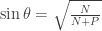
So now we just need to calculate \theta again. The cosine is easy to find:

\cos \theta = \frac{ P + N - 2 \rho + P - N }{ 2 \sqrt{ P (P + N - 2 \rho) } } = \frac{P - \rho}{ \sqrt{P (P + N - 2 \rho) } }.

Then solving for the sine:

\sin^2 \theta = 1 - \frac{ (P - \rho)^2 }{ P( P + N - 2 \rho) }

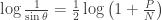
and applying our formula, for \rho < \sqrt{PN},

\log \frac{1}{\sin \theta} = \frac{1}{2} \log\left( \frac{ P ( P + N - 2 \rho) }{ P (P + N - 2 \rho) - (P - \rho)^2 } \right) = \frac{1}{2} \log\left( \frac{ P (P + N - 2 \rho) }{ PN - \rho^2 } \right)

If we plug in \rho = 0 we get back the AWGN capacity and if we plug in \rho = N we get the rate distortion function, but this formula gives the capacity for a range of correlated noise channels.

I like this geometric interpretation because it's easy to work with and I get a lot of intuition out of it, but your mileage may vary.

Advertisement